This is a course project for the “Statistical Methods for Discrete Response, Time Series, and Panel Data (W271)” class at UC Berkeley’s Master in Data Science program. The project team included Sean Seneviratne, Trevor Dalton, Kyle Ruan and Artem Lebedev. Project GitHub repo
The goal of this project was to develop proficiency in building optimal models for time series, including finding the balance between model complexity and robustness. To that end, we were tasked to determine if there is enough evidence that the recent rise in atmospheric carbon dioxide is the result of a larger trend or could be explained by natural variation. Additionally, we were tasked to make several predictions from the perspective of a scientist in 1997 and then evaluate/update these predictions from a 2020 perspective.
Keywords: Time Series Forecast, SARIMA, ACF, PACF, Bayesian Information Criterion, Prediction Confidence Interval, R, tidyverse, ggplot.
Intro
The rise in atmospheric carbon dioxide is often linked to the ongoing global climate change. Given the intensity of societal debate around this issue, credible projections of the future levels and elucidation of the existing trends are needed to further the ongoing environmental debate.
Carbon dioxide measurements from a laboratory at Mauna Loa, Hawaii is the most authoritative data set in the world. This site has been collecting CO2 longer than any other site in the world. It is also unique in that it is representative of air for the entire Northern Hemisphere as it is not affected by nearby vegetation as the site is surrounded by lava flows. All in all, the Mauna Loa data is the gold standard of atmospheric carbon measurements and we will use this data for our analysis
Data and EDA
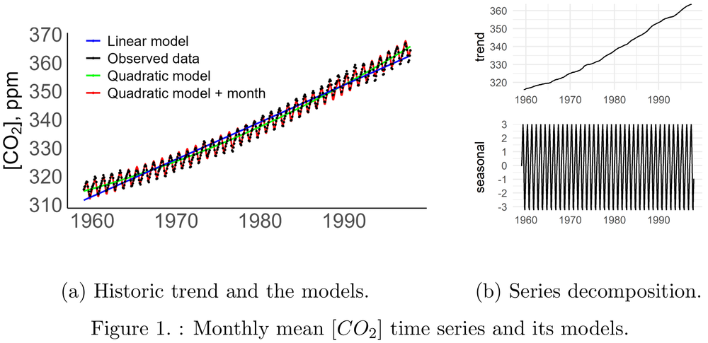
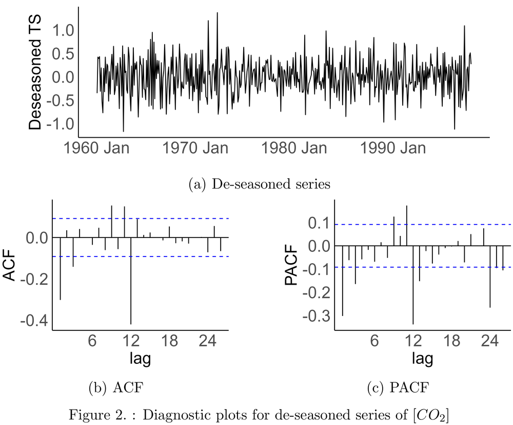
Figure 1 shows observed data (along with some models that will be described later). After removing yearly variability by differencing with a lag of 12 months, the series remains non-stationary, with a visible upward trend. Further de-trending with lag 1 brings it close to stationary (Figure 2a). ACF plot (Figure 2b) shows significant peaks only at lags 1 to 3 and few peaks around lag 12, without a slow-decaying pattern. This indicates an MA(3) process and the need for a seasonal component in SARIMA model. PACF plot (Figure 2c) has a few significant peaks up to lag 3 and a cluster of significant peaks at lag 12. These features indicate the AR(3) process and highlight the need for a seasonal component in the SARIMA model. A grid search of model parameters, including differencing parameters, will be required for precise model allocation.
Baseline: polynomial regression with categorical month variable
Due to the visible non-linearity of the trend we started by estimating a quadratic model This model captured the inherent non-linearity of the trend but failed to capture seasonality. Residuals of this model were not normally distributed and ACF plot exhibited strong osculations
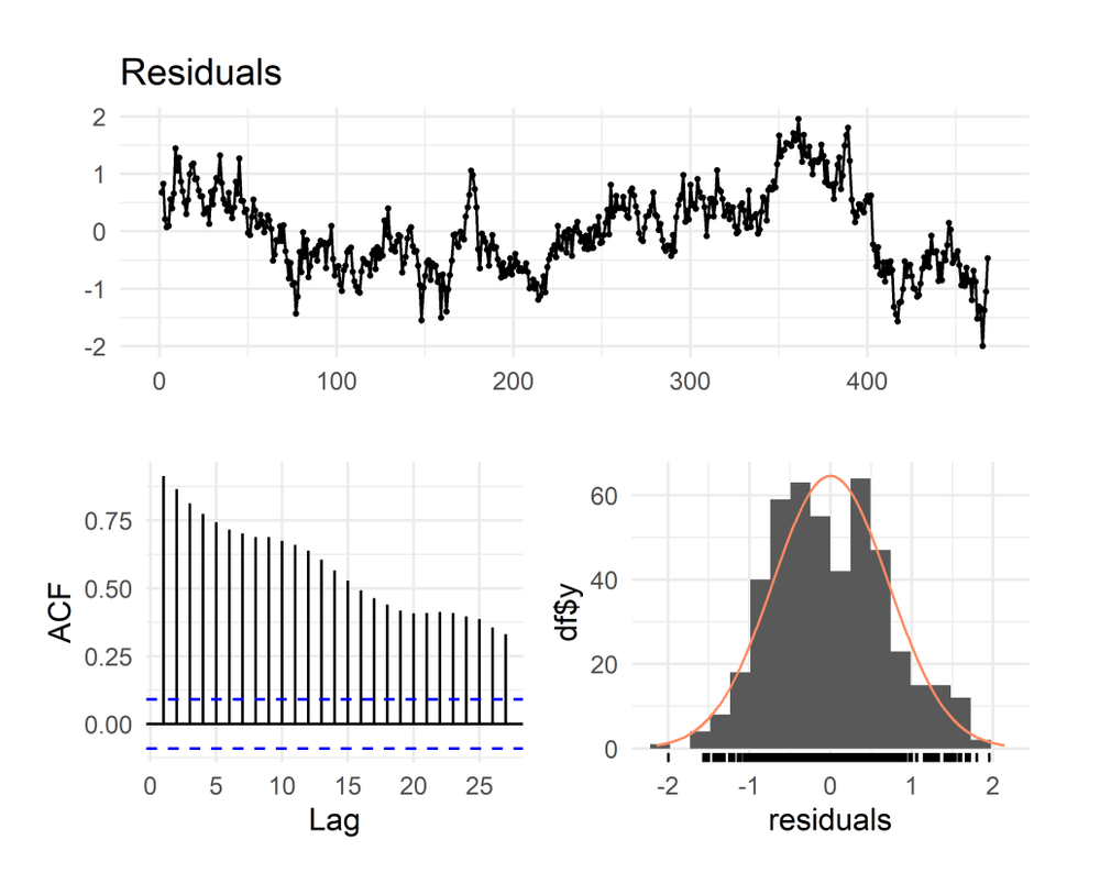
To address the issue of seasonality, we estimated a quadratic model augmented with the variable for the month. Figure 1a show that the use of monthly dummy variables is a marked improvement over the linear and quadratic models, although it does not entirely capture the seasonality the data. Nevertheless, the residuals plot reveals that residuals of this model, although close to normally distributed, are far from white noise. Gradually decaying ACF plot indicates a substantial AR component in the residual series.
SARIMA
Model development
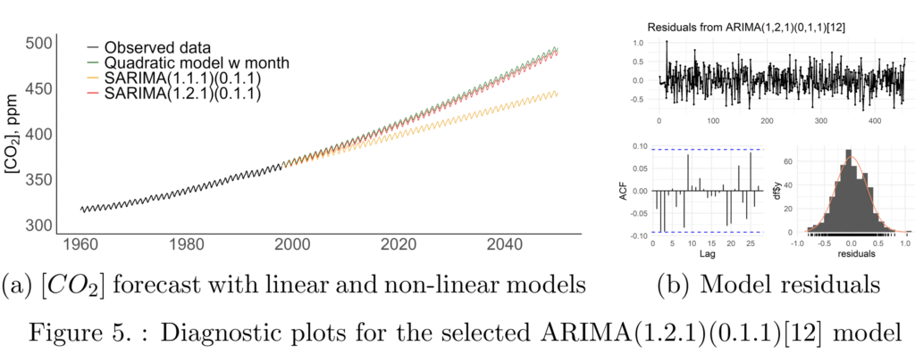
We started developing SARIMA model by de-seasoning of the data by differencing with lag 12, followed by a grid search of ARIMA models, selecting the model with the lowest BIC. The search yields ARIMA(1.1.1) as the preferred model for de-seasoned data. We then fit a few SARIMA models to the original time series, only changing parameters in the range PDQ(0.0.0) to PDQ(2.2.2), again choosing the model with the lowest BIC. This way we arrived at SARIMA(1.1.1)(0.1.1)12 that has BIC of 180.7. However, this model fails to capture the non-linearity that we discovered in the analysis of polynomial models. Figure 5a shows that its predictions continue almost linearly.
To remedy this issue, we introduced double-differencing hoping it would eliminate growth acceleration, similar to how the second derivative of distance over time removes acceleration. Following this line of thought we selected SARIMA(1.2.1)(0.1.1)12 as our final model. This update increased BIC to 216, which we consider a reasonable sacrifice to capture non-linearity. Figure 5b shows that the ACF of the residuals does not have significant values and residuals are close to normally distributed, indicating reasonable quality of the model.
Forecast from 1997 perspective
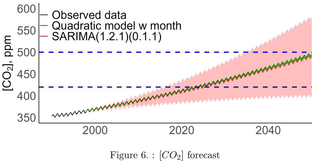
Based on the chosen model, we can attempted to predict some important milestones. For the year 2100, we expect [CO2 ] to be 676 ppm with 95% CI from 391 ppm to 962 ppm. 420 ppm threshold is expected to be crossed on 2024-02-01, but can be crossed as early as 2015-05-01 . 500 ppm thresholds might be crossed as early as 2034-05-01, but most likely on 2053-01-01. Fast-increasing uncertainty in predictions, typical for SARIMA models, limits our ability to make meaningful predictions about the distant future. For instance, despite fast-growing trend, the model can not exclude the possibility that atmospheric CO2 will never exceed 420 and 500 ppm
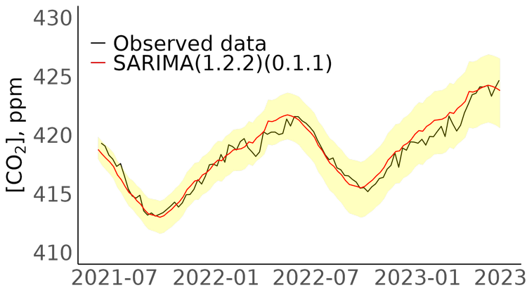
Forecast validation from 2020
perspective
Based on the chosen model, we can attempted to predict some important milestones. For the year 2100, we expect [CO2 ] to be 676 ppm with 95% CI from 391 ppm to 962 ppm. 420 ppm threshold is expected to be crossed on 2024-02-01, but can be crossed as early as 2015-05-01 . 500 ppm thresholds might be crossed as early as 2034-05-01, but most likely on 2053-01-01. Fast-increasing uncertainty in predictions, typical for SARIMA models, limits our ability to make meaningful predictions about the distant future. For instance, despite fast-growing trend, the model can not exclude the possibility that atmospheric CO2 will never exceed 420 and 500 ppm
Conclusions
In this report, we assessed data from the Mona Loa observatory to model and predict atmospheric CO2 concentrations. The forecast from our modeling is only valid assuming all forces that currently influence atmospheric carbon remain unchanged. Surprising performance of our model, that was able to predict with high accuracy CO2 levels 25 years into the future, this assumption is valid. This indicates that no effective action against carbon dioxide emissions has been taken over the past 25 years.